An Introduction to Neural Networks: The Perceptron
Neural networks have come to dominate modern machine learning. Neural networks initially attracted significant press because of their relationship to the human brain enabling the anthropomorphism of artificial intelligence. More recently, their significant successes have given them and machine learning much more prominence. In this post, we take a look at the building block of neural networks, the perceptron. We first discuss the neuron and the percepton before coding a perceptron and training it. Understanding the perceptron helps us to peer into the black box that large neural networks can appear to be.
This article was originally developed as an IPython notebook. The original code is available here on Google Colab where it can be copied and you can run and edit it yourself. Requirements for local running are available at the end of this post.
As of 2020, humans maintain the edge in the comparison of human and computer intelligence particularly when considering adaptation to multiple tasks. Neural networks aim to emulate the neurons of the brain with perceptrons. A look at the so-called 'wetware' specs of the brain and the hardware specs of computers gives us an idea as to where the differences lie.
The Human Brain
- Neuron Switching Time: \(0.001\text{s}\) (\(1\text{ms}\))
- Number of Neurons: \(100\) billion
- Connections per Neuron: \(10^4-10^5\)
- Scene Recognition Time: \(\sim0.1\ Second\)
A Typical Computer
We may see that computer hardware wins the comparison hands down in switching time and is approaching the brain in terms of number of transistors/neurons on a single processor, but the human brain is more powerful as a general purpose computing unit at the moment. The power of this comes through the connections per neuron. It is currently not foreseen that computing hardware of the current paradigm will ever overtake the brain in this respect. The connections between neurons (albeit slow, exchanging information via synapses) are where the brain learns and maintains its computational superiority. However, the figures for hardware will soon be out of date as development continues, in some cases taking inspiration from biology to increase connections between transistors as computers vie for processing superiority.
Perhaps the most significant comparison is the power consumption of the brain. The brain demonstrates amazing processing capacity with power consumption on the order of 100 Watts. Contrastingly, the computers used to train and build the leading neural network models consume far more energy. The brain manages to achieve massive parallelism through the connections of neurons from one to another and thereby achieves remarkable efficiency and intelligence.
The Neuron and the Perceptron
The software equivalent of the neuron is the perceptron. A single neuron is able to encode a single binary threshold which could be sufficient for a simple binary classification model. Neurons fire at a certain rate which is modulated by the incoming signals. To simplify discussion, we consider the binary fire/don't fire boundary which akin to considering a very short timescale. When a neuron 'fires', an action potential is sent down the axon and down the dendrites which then passes the stimulus on to the neurons connected to the neuron in question. The trigger threshold will differ from neuron to neuron as will the number and paths of the connections between neurons. The strength and efficiency of the signal passing is affected by myelination which is thought to be a key process in biological learning.

The perceptron tries to emulate this mathematically by taking in a series of inputs summing them (scaled by some weights) and comparing them to a threshold. It is through updating these weights that a perceptron learns.
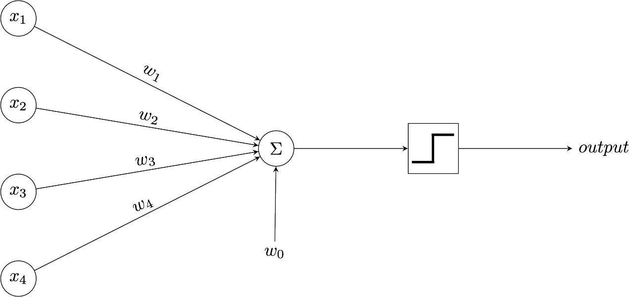
In the diagram the activation threshold is essentially shifted by the learned parameter \(w_0\) which is also referred to as the bias. The inputs are given by the \(n\)-vector \(\boldsymbol{x}\). The \(x\) values are then multiplied by their respective weights and summed before the result is passed through the step function which then leads to a binary output (\(1\) 'fire' or \(0\) 'do not fire'). This step function is known as the activation function since it determines the rule as to whether or not the perception 'fires' (i.e. is activated). Usually, when building neural networks, this activation function can be chosen and is typically differentiable and non-linear. We'll cover activation functions in a later post.
Mathematically the perceptron (in the case of the purest neuron emulation) undertakes the following calculation:
$$output = \begin{cases} 1 &\mbox{if } \left(w_0 + \sum_{i=1}^n w_ix_i\right)>0 \\ 0 & \mbox{otherwise} \end{cases}$$
In this way a perceptron learns a hyperplane which divides its input space in two.
The output of a perceptron or a set of perceptrons can be passed forwards to other perceptrons akin to the action potential passing from the dendrites of one neuron to the next neuron through the chemical mediation of a synapse (which is very slow by computing standards). In this way perceptrons are built up to generate a neural network. We may now understand that the power of neural networks comes from hierarchically building up the classifying hyperplanes from each perceptron to form a more complex yet fully learnable function.
Taking the single perceptron as an example we may see that the hyperplane it characterises implements binary classification. The gradient of the hyperplane is determined by the weights vector \(\boldsymbol{w}\) and its position is given by the bias \(w_0\). The two-dimensional case leads to classification according to a single straight line which clearly shows the limitations of the perceptron as a classifier - it can only separate two regions and only then in a linear way. The most oft-cited example of what such linear separation cannot deal with is the case of parity (a.k.a. the exclusive-or or XOR function). However, we will see later that neural networks can get around this issue thanks to multiple layers of perceptrons.
The 'learning' of anything in neural networks is mediated through the weights. The weights encode all knowledge. The learning process begins with the weights initialised at small random numbers and then as examples are seen and errors noted the weights are updated in order to reduce the error. This can be thought of as the strengthening of pathways in the brain. The more a path is used to predict the output the greater the magnitude of the weight of that link in the network. Different paths may be activated for different inputs allowing for classification. This comparison is more clear-cut in the case of a neural network where the inputs to one perceptron are the outputs of other perceptrons.
Coding a Perceptron
We will use Python to set up a perceptron and gain an idea of how to train it. To do this we will use NumPy, the go to package for scientific computing in Python.
There are many packages for building neural networks in Python popular choices being SciKit-Learn, Keras, PyTorch, JAX and TensorFlow however we will initially build our models from scratch using standard mathematical libraries (see below) for pedagogic suitability.
import numpy as np
import pandas as pd
In keeping with the idea that a perceptron simply learns a hyperplane we will set up a dataset that classifies points based on a hyperplane. We will then try to learn the formulation of this hyperplane with a single perceptron.
Creating a Dataset
To set up the dataset we will simply take points in three-dimensional space and classify them according to the hyperplane defined below. Below the hyperplane the points will be coded as -1 and above they will be encoded as 1.
$$-1.8x + 0.7y + 2.1z = 0.5$$
The dataset will be created from random values in the unit interval for \(x, y\) and \(z\).
x = np.random.uniform(size=(5000))
y = np.random.uniform(size=(5000))
z = np.random.uniform(size=(5000))
output = -1.8 * x + 0.7 * y + 2.1 * z > 0.5
output = 2 * output.astype(np.float32) - 1
All being well, the dataset should yield approximately 32% positive and 68% negative outcomes. Let us place all of the data in a Pandas DataFrame so that we may view and manipulate the data in tabular form.
data = pd.DataFrame(data={'x':x,'y':y,'z':z,'Target':output})
data = data[['x','y','z','Target']]
data.head()| x | y | z | Target | |
|---|---|---|---|---|
| 0 | 0.379099 | 0.314081 | 0.025111 | -1.0 |
| 1 | 0.567098 | 0.319218 | 0.060301 | -1.0 |
| 2 | 0.595593 | 0.249794 | 0.552818 | -1.0 |
| 3 | 0.449859 | 0.087631 | 0.784544 | 1.0 |
| 4 | 0.457020 | 0.036829 | 0.926797 | 1.0 |
Now that we have our dataset and an idea of the target function, we may set up our perceptron. We initialise the weights vector to small random values. For simplicity we then build a function which will generate a prediction given the input vector and weights vector which includes the bias (hence why it is of size NUM_INPUTS + 1). The weights vector is initialised to small random values as we do not wish to impose any significant initial model or relationship before the model has been shown data.
NUM_INPUTS = 3
weights = w = np.round(np.random.normal(size=NUM_INPUTS + 1, scale=0.5), 2)
When generating a prediction, we must generate a binary output. This is done by comparing the sum of the product of the weights and the inputs to the threshold. This threshold is effectively learned through the bias \(w_0\). We prepend a \(1\) to the input vector to account for the bias. Note that this means that the bias is therefore entering additively and will be learned as the negative of the value used in constructing the data set. Including the bias in the weights vector enables classification via a generic comparison to \(0\) as the bias is already accounted for in the dot product of inputs and weights.
def perceptron_prediction(input_vector, weights):
    inputs = [1, *input_vector]
    prediction = 2 * float(np.dot(weights, inputs) > 0) - 1
    return prediction
If the perceptron manages to learn the model exactly then we will expect the following weights vector (or a non-zero multiple thereof).
$$\boldsymbol{w}=\begin{bmatrix}w_0 \\ w_1 \\ w_2 \\ w_3\end{bmatrix}= \left[ \begin{matrix} -0.5 \\ -1.8 \\ 0.7 \\ 2.1 \end{matrix} \right]$$
Perceptron Training
In machine learning, as in life, we learn from our mistakes. Models are improved by identifying errors and reducing them by manipulating the parameters of our model. In the case of the perceptron, we will update our weights to reduce the prediction error.
The weights are first initialised to small non-zero values. They must be non-zero as all zero entries will lead to a zero output regardless of inputs and therefore the initial step does not enable us to distinguish between which weights are most responsible for the initial inaccuracy. We also initialise to random small numbers so as not to impose any significant presupposed relationship to start learning from (as would be the case with large or non-random weight initialisations). The use of randomness means that our model may converge to a different result in the case that there are local minima rather than finding the true global optimum. Running several training sessions with random initialisations can enable comparison of final models to hopefully find the global minimum for the loss function.
The Perceptron Training Rule
As one may expect given the explanation above, the perceptron training rule relates the weights update to the size of the error, the learning rate (\(\eta\)) and the nature of the input (\(\boldsymbol{x}\)). The weights are updated in turn by the required change \(\Delta w_i\) where the update is as given below.
$$\Delta w_i=\eta\ (t - o)\ x_i$$
Where \(\eta\) is the 'learning rate', \(w_i\) is the weight being trained, \(t\) is the target value (i.e. the label for this observation), \(o\) is the output of the perceptron with the current weights and \(x_i\) is the \(i^{th}\) element of the input vector \(\boldsymbol{x}\) which, when scaled by \(w_i\), contributes to the generation of the output \(o\).
The error term \((t - o)\) ensures that the weights are only updated if they need to be and indeed in the case that they are updated they should be updated in the right direction. The inclusion of the input element \(x_i\) further ensures that learning occurs in the right direction since inputs may in practice be positive or negative. Since the weights enter the prediction equation multiplicatively, the sign of the inputs is important in determining the sign of the influence on the output.
The size of the learning rate is one of the hyperparameters that one can play with to improve one's model. Since the learning rate \((\eta)\) determines the size of the step taken towards the minimum, we may understand that too large an \(\eta\) will lead to potentially overshooting the global minimum and not being able to reach it with sufficient precision (only being able to attain final weights with a precision of \(\eta\)). Too small a learning rate, \(\eta\) may lead to very slow convergence if the initialisation is far from the optimum. Furthermore, in the case of real noisy data the model is likely to overfit if trained for many iterations with a small learning rate (allowing for fine-grained changes).
Overfitting is a major concern in machine learning. It is the problem of learning and then drawing on relationships in the training data that are specific to that sample and not generally applicable to the population as a whole. This will lead to in-sample tests showing high accuracy but when applied to out-of-sample cases the model is inaccurate since the special case relationships of the sample no longer hold true.
In the rare case that the relationship is not noisy (i.e. when modelling unknown yet deterministic processes), we may be less concerned with overfitting since there is no noise to erroneously fit to (although there is still the concern of non-representative sampling of training data). In the case presented here, there is no noise in the data and we have a sufficiently large training set. Hence, we choose a small value of \(\eta\) to hopefully get close to learning the true underlying relationship.
In practical applications, decades of field experience and research has led to the rule of thumb that a learning rate of \(0.1\) is generally a good place to start when training perceptrons with noisy data.
Stochastic Gradient Descent
Stochastic Gradient Descent is a general and powerful learning algorithm that is able to cope with learning with continuous variables over many dimensions. This generality comes at a cost of increased complexity when compared to perceptron training, but it is still intuitive. It is only required that the objective be differentiable.
We aim to minimise the loss from our prediction algorithm. This loss can take many forms but should be decreasing in the accuracy of our model. Let us aim to minimise the mean squared error from our predictions (scaled by \(\frac{1}{2}\) to simplify the later mathematics without changing the dynamics of the problem). Let us consider this for all data points in our dataset; \(d \in D\).
$$loss\ (\boldsymbol{w}) = \mathbb{E}[\boldsymbol{w}]=\frac{1}{2}\sum_{d\in D} (t_d - o_d(\boldsymbol{w}))^2$$
This therefore makes the optimisation problem to be solved:
$$\min_{\boldsymbol{w}}\ \mathbb{E}[\boldsymbol{w}]=\frac{1}{2}\sum_{d\in D} (t_d - o_d(\boldsymbol{w}))^2$$
Note: We have divided the error by two to simplify later mathematics. This coefficient is constant and therefore does not change the optimal solution to the minimisation problem in terms of the weights \(\boldsymbol{w}\).
The weights of the perceptron are denoted by \(\boldsymbol{w}\), the target value (label) for each example $d$ by \(t_d\) and the predicted value from the model by \(o_d\). The error for example $d$ is therefore given by \((t_d - o_d)\). This error is a function of our weights indirectly since the weights affect the prediction \(o\) and therefore influence the error in this way.
The termination condition is best described using a spatial example. Imagine that the surface of errors given the weights is a valley. At each point in the learning process there is some error at the point in the valley. From this point learning is achieved by taking a step in the downward direction. The fastest way to the bottom of the valley (i.e. the loss minimisation point which minimises the squared errors and therefore is the optimal model characterised by the weights \(\boldsymbol{w}\)) is to head downhill following the steepest path. The slope of any path is given by the derivative of the loss function at the point in question \(\nabla_\boldsymbol{w} loss(\boldsymbol{w})\). The learning therefore ends (i.e. weights no longer change) when all neighbouring points are weakly above the current position (or more often within some tolerance below the current point).
Note that this may not necessarily mean that the true optimum has been found, simply a local one. For example, over the next ridge may be a deeper valley (i.e. the potential to improve the model and further reduce the error). We can never fully map the loss surface. Initialising the training several times from random starting points and even roughly mapping the loss surface using some random searching functionality can aid in giving confidence that we have found the best feasible model given our hypothesis space (the space of possible models given the initial model architecture).
Before we define the training rule, let us first define the gradient of the loss function as follows:
$$\nabla\mathbb{E}[\boldsymbol{w}]\equiv \left[\frac{\partial\mathbb{E}}{\partial w_0},\frac{\partial\mathbb{E}}{\partial w_1}, \cdots \frac{\partial\mathbb{E}}{\partial w_n}\right]$$
Having defined this gradient vector, we may now define the training rule.
$$\Delta w=-\eta\ \nabla\mathbb{E}[\boldsymbol{w}]$$
Note the negative sign since we aim to reduce the error and therefore follow the function down rather than up ('upwards' and 'downwards' being denoted by positive and negative values respectively).
\(\eta\) again denotes the learning rate.
In the case of an individual weight \(w_i\) we attain the following learning rule.
$$\Delta w_i = -\eta\ \frac{\partial \mathbb{E}}{\partial w_i}$$
Applying this to our mean squared error loss function (assuming that the input vector is prepended with an entry of \(1\) to handle the intercept weight). We attain:
$$ \begin{align} \frac{\partial\mathbb{E}}{\partial w_i} &= \frac{\partial}{\partial w_i}\ \frac{1}{2}\sum_{d\in D}(t_d - o_d)^2\\&=\frac{1}{2}\sum_{d\in D}\frac{\partial}{\partial w_i}(t_d - o_d)^2\\&=\frac{1}{2}\sum_{d\in D}2(t_d - o_d)\ \frac{\partial}{\partial w_i}(t_d - o_d)\\&=\sum_{d\in D}(t_d - o_d)\ \frac{\partial}{\partial w_i}(t_d - \boldsymbol{w}\cdot\boldsymbol{x})\\&=\sum_{d\in D} (t_d - o_d)(-x_{i,d})\\&=-\sum_{d\in D}x_{i,d}(t_d - o_d) \end{align} $$
Given that we aim to fit a precise relationship with clean data we set a relatively low learning rate \(\eta = 0.001\) this will mean that we iterate slowly to a solution, but we should end with a very accurate classifier.
eta = 0.001To measure the progress towards a perfect classifier let us generate an accuracy measure.
Each example is given in the list rows. We compare the prediction from our current perceptron with the true label values. We then give our accuracy as 1 less the error rate. This function therefore returns the percentage of correct predictions managed by the current perceptron (i.e. the weights at the current point in learning).
def accuracy(data, weights, prediction_fn):
    x = data.copy()
    y = x.pop(x.columns[-1])
    rows = np.array([*x.itertuples(index=False)])
    predictions = np.array([prediction_fn(input_x, weights) for input_x in rows])
    errors = np.abs(y - predictions)/2
    accuracy = 1 - errors.mean()
    return accuracy
Now the key to machine learning - the learning. We keep track of the accuracy throughout the training process to enable us to plot the progress later. Given our low learning rate and limited data size we will pass over the data several (6) times in order to learn from each data point at different stages towards our final model.
For each data point we apply the learning rule to attain the weight update (line 12).
$$\Delta\boldsymbol{w}=\eta\ \boldsymbol{x}\ (y_d - o_d)$$
You should be able to see the progress in terms of prediction accuracy printed out as the learning progresses. This relationship between training period and accuracy is plotted later.
def train_perceptron(prediction_fn, data, eta, weights, repeats=6):
    accuracy_trajectory = []
    training_data = data.copy()
    epochs = len(training_data) * repeats
    w = np.copy(weights)
    for epoch in range(epochs):
        example = training_data.iloc[epoch % len(data)]
        x = example[:-1]
        y = example[-1]
        prediction = prediction_fn(x, w)
        updates = eta * np.array([1, *x]) * (y - prediction)
        w += updates
        if epoch % 50 == 0:
            current_accuracy = accuracy(training_data, w, prediction_fn)
            print('Epoch {0}: Current accuracy: {1:.2%}'.format(epoch, current_accuracy), end='\r')
            accuracy_trajectory.append(current_accuracy)
    final_accuracy = accuracy(training_data, w, prediction_fn)
    accuracy_trajectory.append(final_accuracy)
    print('Epoch {0}: Final accuracy: {1:.2%}'.format(epochs, current_accuracy), end='\r')
    return w, accuracy_trajectory
Having set everything up, let us train our model using the data. This should result in accuracy of around 99%.
w, accuracy_trajectory = train_perceptron(perceptron_prediction, data, eta, weights)Epoch 30000: Final accuracy: 99.92%
Now we may plot the progress of our learner. We use the standard libraries of matplotlib and seaborn styling.

Note that beyond 20,000 updates there is little, if any, more learning achieved. The accuracy rate does however still change. This tells us that we do not have a perfect classifier as at such a point there would be no more changes as the update rule would lead to 0 update values. This tells us that the learning rate is leading the perceptron to jump over the optimal values and fluctuate around the optimum. A smaller learning rate may lead to a better classifier in this case, but it will take much longer to arrive at a final trained model.
We may see from the below that the best our model achieved was 99.92% accuracy meaning that of our 5,000 data points all but 4 were classified correctly.
max(accuracy_trajectory)0.9992
Updates leading to worse models as observed towards the end of training will be caused by updates being too large (due to the size of the learning rate). This shows us that there must be several points close to the plane on each side such that even small updates affect their classification and therefore influence the overall error rate.
As a verification exercise let us check that the accuracy with the parameters used to construct the data set is 100%. We may see by the check below that it is indeed.
true_weights = np.array([-0.5, -1.8, 0.7, 2.1])
accuracy(data, true_weights, perceptron_prediction)
1.0
We may now look at the weights that we learned from the model. Remembering that the 'correct' weights will be any positive multiple of the true weights. We may see from the calculation below that our weights are approximately equal to 0.23 times the values used in generating the dataset.
The values will only be exact in the case that our data set is sufficiently large, our learning rate sufficiently small (and with enough training to allow for convergence) and if the training data contains points within some very small margin (\(\varepsilon\)) of the plane separating positive and negative data points as these points enable the pinning down of the weights more exactly.
warray([-0.116 , -0.41973931, 0.16399407, 0.48946506])
w/true_weightsarray([0.232 , 0.2331885 , 0.23427725, 0.2330786 ])
For future analysis let us augment our dataset by creating a new DataFrame which includes model predictions and errors. We do so using our current weights and making the most of Pandas' DataFrame functionality.
def append_predictions_and_errors(df, prediction_fn, weights):
    x = data.copy()
    y = x.pop(x.columns[-1])
    rows = np.array([*x.itertuples(index=False)])
    predictions = np.array([prediction_fn(input_x, weights) for input_x in rows])
    errors = y - predictions
    output = df.copy()
    output['Prediction'] = predictions
    output['Error'] = errors
    return output
df = append_predictions_and_errors(data, perceptron_prediction, w)Having created this new dataframe we may look only at the misclassified examples and see how many times (out of 5,000) our perceptron is incorrect.
errors_df = df[df.Error != 0]
len(errors_df)
4
Improving the model
Having trained the model once and having seen the learning plateau in efficacy, we may try to improve using a smaller learning rate to try and iterate towards perfection. This should lead us towards 100% accuracy.
This works here because there is no noise in our data to overfit to and a smaller learning rate means that each update is smaller and hence a finer change in the learned plane is made meaning that we may get closer to the optimum since the adjustments are more fine-grained and we can be more precise in estimating the true plane. We also know that the underlying data set is separated by a plane therefore we are using a model that can exactly fit the underlying relationship. That is to say that we have a rare certainty that the true relationship does indeed lie in our hypothesis space (the space of all possible model outputs, given our chosen model architecture).
eta_small = 0.00005
w, extended_accuracy_trajectory = train_perceptron(perceptron_prediction, data, eta_small, w)
Epoch 30000: Final accuracy: 100.00%
Plotting the results
Now let us use plotly to see what we have achieved.
Plotly uses D3.js under the covers to generate interactive web-based charting. The chart we create will be interactive allowing the viewer to zoom in and rotate the plot. (We use offline mode so that we can keep JavaScript is kept within the generated HTML plot rather than calling out to external sources.)
import plotly
import plotly.plotly as py
import plotly.graph_objs as go
plotly.offline.init_notebook_mode()
To generate the true separating plane, we define the function implementing the equation of the plane below.
This is defined using the lambda shorthand which takes in \(x\) and \(y\) and returns us \(z\).
$$z = \frac{0.5 + 1.8x - 0.7y}{2.1}$$
f = lambda x, y: (0.5 + 1.8*x - 0.7*y)/2.1domain = np.linspace(0,1,101)
z = f(*np.meshgrid(domain, domain))Having defined our plane we take a sample of our data set and split them according to positive and negative points so that we may plot them in different colours to emphasise the divide between the positive and negative points.
sample = data.sample(250)
above = sample[sample.Target==1]
below = sample[sample.Target==-1]
above_x = above.x
above_y = above.y
above_z = above.zbelow_x = below.x
below_y = below.y
below_z = below.zFor comparison we also want to plot the plane that we have learned to see how it differs from the true plane we were aiming for. This uses the same implementation style as was used for generating the points of the true plane.
def generate_plane_from_weights(weights, domain):
    points = np.meshgrid(domain, domain)
    f = lambda x, y:  (-weights[0] - weights[1] * x - weights[2] * y)/weights[3]
    return f(*points)
learned_plane = generate_plane_from_weights(w, domain)Finally, let us regenerate our data frame containing the predictions and errors from our improved model. This will then enable us to plot the points which we are still misclassifying to see why they may be misclassified.
augmented_df = append_predictions_and_errors(data, perceptron_prediction, w)
errors = augmented_df[augmented_df.Error != 0]
errors_x = errors.x.values
errors_y = errors.y.values
errors_z = errors.z.values
charts = [
go.Surface(x=domain, y=domain, z=z, colorscale=[[0, 'gray'], [1, 'gray']],
showscale=False, cauto=False, opacity=0.95, name='True Boundary'),
go.Surface(x=domain, y=domain, z=learned_plane, colorscale=[[0, 'purple'], [1, 'purple']],
showscale=False, cauto=False, opacity=1, name='Learned Boundary'),
go.Scatter3d(x=above_x, y=above_y, z=above_z, showlegend=False, mode='markers', name='Positive Example',
marker=dict(color='rgb(128,0,0)',size=4,opacity=0.75)),
go.Scatter3d(x=below_x, y=below_y, z=below_z, showlegend=False, mode='markers', name='Negative Example',
marker=dict(color='rgb(0,0,128)',size=4,opacity=0.75)),
go.Scatter3d(x=errors_x, y=errors_y, z=errors_z, showlegend=False, mode='markers', name='Incorrect Classifications',
marker=dict(color='rgb(255,191,0)',size=8,opacity=1))
]
layout = go.Layout(width=1000, height=600, margin=dict(l=0, r=0, b=65, t=90), paper_bgcolor="rgba(0,0,0,0)")
fig = go.Figure(data=charts, layout=layout)
plotly.offline.iplot(fig)The positive points are marked in red, the negative in blue and the errors in orange alongside the true plane marked in grey and the estimated plane marked in purple.
We may see that we have almost perfectly matched the true plane and the few errors are very close to the true plane. This therefore shows the efficacy of our model and how hard it can be to separate even a clean data set using machine learning. In this case we have achieved very high accuracy but not perfect accuracy despite having a deterministic relationship to fit to.
The error points will have been learned from, but they are so close to the plane that even with the smaller learning rate our model was unable to update itself finely enough to correctly classify these points.
Conclusion
We have considered some of the parallels of deep learning and the working of the human brain from the perspective of their fundamental building blocks, the neuron and the perceptron. We implemented a perceptron in python and trained it using stochastic gradient descent. We visualised progress towards perfect training performance and discussed some of the issues of overfitting and fine tuning models.
We may now understand how neural networks are able to learn complex functions by connecting and stacking layers of perceptrons together. The plane learned by our simple classifying perceptron when combined with many other planes and multiple layers of processing could separate the input space into much more complex shapes. For this reason, neural networks are sometimes referred to as universal function approximators.
Much of modern machine learning research considers the choice of how many perceptrons to put in a layer of a neural network, how many layers to use, which activation functions to use, how to connect the layers, which loss to use along with many other questions and how their answers affect the dynamics and efficacy of learning. In later posts we will come to these questions. To understand the possible answers, our understanding of the primary building block, the perceptron, will be highly valuable!
Code Requirements
When writing the code for this article we used Python 3.8.6. The relevant package versions are given below.
matplotlib==3.3.2
numpy==1.18.5
pandas==1.2.0
plotly==4.14.1
seaborn==0.11.1